Sensor Foundations · Module 1 — Measurement
How Sensors Turn the Physical World Into Data
Every measurement is a translation. This lesson follows a physical quantity from the world, through a transducer and an analog front end, into numbers you can trust — and shows exactly where that trust is won or lost.
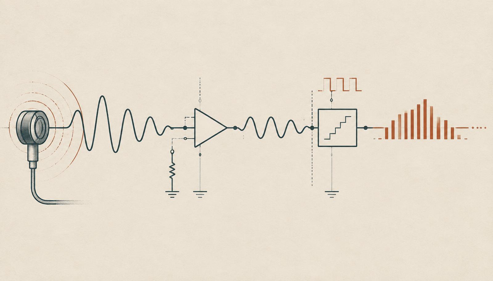
Sensing feels like observation, but it is really translation. Nothing about a roast, a bearing or a bioreactor is inherently numeric. A sensor imposes a numeric description on a physical situation, and everything downstream — your filters, your features, your model, your control loop — inherits the quality and the assumptions of that translation.
This lesson walks the whole chain once, slowly, in the order the physics actually happens: measurand, transducer, transfer function, conditioning, digitisation, and finally the maintenance work of calibration. By the end you should be able to sit with an instrumentation engineer and ask the two questions that matter most: what exactly are we measuring, and how wrong could this number be?
1. Start with the measurand, not the sensor
The measurand is the physical quantity you actually care about. Naming it precisely is the single highest-leverage act in any sensing project, because vague measurands produce systems that appear to work and then fail in ways no one can debug.
Consider "steak temperature". That phrase hides at least four distinct measurands: surface temperature of the crust, temperature at the geometric centre, the volume-average temperature, and the temperature at the thermal centre — which is not the geometric centre in an irregular cut. A thermal camera measures the first. A probe measures whatever the tip happens to touch. A model can estimate the third. Confusing them is not a small error; it is a category error that propagates into every label in your dataset.
2. The transducer: where physics becomes signal
A transducer converts energy from one domain into another. Almost all practical sensing reduces to a handful of physical effects, and knowing which one you are relying on tells you where the sensor will misbehave.
| Effect | Physical mechanism | Typical sensor | Where it breaks |
|---|---|---|---|
| Resistive | Resistance varies with temperature or strain | RTD, thermistor, strain gauge | Self-heating, lead resistance |
| Thermoelectric | Junction of dissimilar metals generates voltage | Thermocouple | Cold-junction error, tiny signals |
| Piezoelectric | Mechanical stress generates charge | Accelerometer, ultrasonic transducer | No true DC response, charge leakage |
| Capacitive | Geometry or dielectric changes capacitance | Pressure, humidity, MEMS mics | Stray capacitance, condensation |
| Photoelectric | Photons liberate charge carriers | Image sensor, photodiode | Dark current, saturation |
| Chemiresistive | Adsorbed gas changes surface conductivity | MOX gas sensor | Cross-sensitivity, poisoning, drift |
Diagram · Measurand → transducer → analog front end → ADC → digital domain
3. Transfer functions, sensitivity and linearity
The transfer function maps measurand to output. In the friendly case it is a straight line: output equals offset plus sensitivity times input. Sensitivity is the slope — millivolts per newton, counts per degree, nanoamps per ppm.
Real devices deviate. A thermistor is strongly exponential. A load cell is close to linear but shows a small non-linearity plus hysteresis. A MOX gas sensor follows roughly a power law in concentration and shifts with humidity. Two consequences follow. First, you must know the working range where your linear assumption is acceptable. Second, the correction you apply — polynomial fit, Steinhart–Hart equation, lookup table — becomes part of your instrument and must be versioned like code.
# Converting raw ADC counts to physical units, explicitly.
V_REF = 3.300        # volts, the ADC reference
BITS  = 12           # ADC resolution
GAIN  = 101.0        # instrumentation amplifier gain
SENS  = 0.0020       # sensor sensitivity, volts per unit measurand
OFFSET = 0.0125      # measured zero-point output, volts

def counts_to_units(counts: int) -> float:
    v_adc = counts * V_REF / (2 ** BITS - 1)   # volts at the ADC pin
    v_sensor = v_adc / GAIN                    # undo amplification
    return (v_sensor - OFFSET) / SENS          # apply calibration

lsb_in_units = (V_REF / (2 ** BITS - 1)) / GAIN / SENS
print(f"one count is worth {lsb_in_units:.4f} units")4. Signal conditioning: the stage that decides your data quality
Between transducer and converter sits the analog front end. Its job is to present the ADC with a clean, correctly scaled voltage. It usually performs four tasks: amplification of small signals, buffering so the sensor is not loaded, filtering to remove content you cannot sample, and level shifting into the converter's input window.
- Amplify early. Noise added after amplification is divided by the gain when referred back to the input; noise added before it is not.
- Match impedance. A high-impedance source into a low-impedance input produces an attenuated, temperature-dependent reading.
- Filter before sampling. An anti-alias filter is analog by necessity — it must act before quantisation.
- Respect the reference. ADC accuracy is measured against its voltage reference; a drifting reference drifts every reading.
- Mind the ground. Shared return paths inject the motor's current into your millivolt signal.
5. Resolution, accuracy and precision are not synonyms
This distinction is where most non-specialists lose credibility in technical conversation, and it is easy to fix.
| Property | Question it answers | Improved by |
|---|---|---|
| Resolution | What is the smallest change I can see? | More ADC bits, higher gain, lower noise floor |
| Precision | If nothing changes, do I get the same number? | Averaging, shielding, thermal stability |
| Accuracy | Is the number close to truth? | Calibration against a traceable reference |
| Trueness of trend | Does it move the right way, by the right amount? | Linearity correction, span calibration |
A 24-bit converter attached to an uncalibrated sensor gives you many digits of a wrong answer. That is often acceptable — for control loops and for machine learning you frequently need consistency more than absolute truth — but it must be a deliberate choice, stated out loud.
Diagram · Four target diagrams: precise+accurate, precise+biased, scattered+centred, scattered+biased
6. Noise, averaging and the limits of cleverness
Noise is the random part of your reading. Thermal (Johnson) noise arises in every resistance. Shot noise arises from the discreteness of charge. Flicker noise dominates at low frequencies and is why slow measurements are surprisingly hard. On top of these sit interference sources that are not random at all: mains hum, switching converters, motor commutation, Wi-Fi radios.
Averaging N independent samples reduces random noise by the square root of N. Ten times quieter costs one hundred times more samples — and the improvement stops the moment the error is systematic rather than random. Averaging never fixes bias, aliasing or drift.
7. Sampling: turning a continuous world into a series
Sampling replaces a continuous signal with values at instants. The Nyquist criterion says you must sample at more than twice the highest frequency present in the signal — present, not present-and-interesting. Content above that limit does not disappear; it folds down and appears as a plausible-looking low-frequency wobble that no downstream algorithm can distinguish from truth.
- 01Identify the fastest real dynamics you must capture (a sizzle transient, a pressure spike, a vibration mode).
- 02Choose an anti-alias filter whose cutoff sits below half your intended sample rate.
- 03Sample comfortably above Nyquist — five to ten times the bandwidth of interest is common engineering practice.
- 04Record the timebase. Jittery, undated samples are far less useful than fewer well-timed ones.
8. Calibration and drift: measurement as maintenance
Calibration establishes the mapping between your sensor output and a reference you trust. A two-point calibration fixes offset and span; multi-point calibration also captures curvature. Traceability means your reference is itself linked, through a documented chain, to a national standard.
Drift is the slow decay of that mapping. Thermistors age. Load cells creep. MOX gas sensors baseline-shift after every exposure and take hours to recover. Camera colour response changes as LEDs age. The professional posture is not to hope for stable hardware but to design for recalibration: reference targets in every image, a known-mass check on the scale each shift, a clean-air baseline for every gas array.
9. Worked example: instrumenting a roast
Take a concrete case relevant to a cooking intelligence system: a chicken roasting in a convection oven. You want to know doneness, surface colour development and when to intervene. Consider what each channel actually measures.
| Channel | Measurand | Honest limitation |
|---|---|---|
| Type-K probe in breast | Temperature at the tip location | Placement error of 8 mm can mean 4 °C; conducts heat along the wire |
| IR thermopile at the surface | Radiometric surface temperature | Depends on emissivity; steam and grease on the window corrupt it |
| RGB camera | Reflected light under oven illumination | Colour shifts with lamp ageing and condensation; needs a grey reference |
| MOX gas array | Mixed VOC concentration, unselectively | Cross-sensitive to humidity; baseline drifts within one bake |
| Load cell under the tray | Total mass, hence cumulative water loss | Vibration from the fan; thermal drift of the bridge |
| Microphone near the pan | Acoustic power of boiling and sizzling | Fan and compressor noise dominate without band selection |
Notice the pattern: no single channel measures doneness. Mass loss gives an integral of evaporation. The gas array senses Maillard progression but not its location. The probe is precise about one point and silent about the rest. Doneness is an inferred state, estimated by combining weak, biased, complementary evidence — which is exactly the argument for sensor fusion in the next lesson.
Diagram · Timeline of a 70-minute roast with probe temperature, mass loss, VOC index and sizzle energy overlaid
10. A short field checklist
- 01State the measurand with units and a location.
- 02Name the physical effect the sensor exploits.
- 03Write down the range, sensitivity and linear region you rely on.
- 04Compute one LSB in physical units and compare it to the effect size you claim.
- 05Identify the dominant noise source and the dominant systematic error — they are rarely the same.
- 06Choose sample rate and anti-alias filter together.
- 07Define the calibration procedure and its interval before collecting a single production sample.
- 08Log metadata: device serial, firmware version, calibration date, ambient conditions.
Recap
A sensor is a translator with a specification, not an oracle. The measurand defines what you are asking; the transducer and its transfer function determine how faithfully it is answered; the analog front end sets the ceiling on quality; sampling decides which dynamics survive; and calibration keeps the whole arrangement honest over time. Every sophisticated technique later in this curriculum — fusion, embeddings, learned models — operates on the residue of decisions made in this chain. Get the chain right and the intelligence layer becomes tractable. Get it wrong and no model can rescue you.
Engineer vocabulary
- Measurand
- The physical quantity you intend to measure — temperature, pressure, gas concentration, strain.
- Transducer
- The element that converts energy from one form to another, e.g. heat into resistance change.
- Transfer function
- The mathematical relationship mapping measurand to output signal, including its slope and curvature.
- Sensitivity
- How much output you get per unit of input — the slope of the transfer function.
- Resolution
- The smallest change the system can distinguish, often set by ADC bits and noise floor.
- Accuracy
- Closeness to the true value, i.e. freedom from systematic error.
- Precision
- Repeatability of readings under unchanged conditions; low random spread.
- Signal conditioning
- Amplification, buffering, filtering and level shifting applied before digitisation.
- ADC
- Analog-to-digital converter — quantises a continuous voltage into discrete counts.
- Aliasing
- High-frequency content masquerading as low-frequency content because sampling was too slow.
- Drift
- Slow change in offset or sensitivity over time, temperature or exposure.
- Hysteresis
- Output depending on the direction of approach, not only the present measurand value.
Key concepts to carry forward
- A sensor is a translator: it converts a physical measurand into a signal governed by a transfer function you must know.
- Resolution, accuracy and precision are three independent properties. A device can be exquisitely precise and consistently wrong.
- Most measurement quality is decided in the analog front end, before a single bit is stored.
- Sampling rate and filtering must be chosen together; a filter after aliasing cannot undo it.
- Calibration is not a one-time factory event but a maintenance schedule against drift.
Questions I should be able to answer
- 01What is the measurand in my system, and what physical effect actually converts it into a signal?
- 02What is the transfer function of my sensor, and over what range is it linear?
- 03If my ADC is 12-bit, what is one least-significant bit worth in physical units?
- 04Where does the dominant noise in my chain come from — the sensor, the amplifier, or the environment?
- 05How would I detect that a sensor has drifted rather than that the world has changed?
- 06What sampling rate does my fastest physical process demand, and what anti-alias filter matches it?
Sources
- Sample citation — instrumentation textbook chapter on measurement chains — Demo reference, 2026
- Sample citation — application note on anti-alias filtering — Demo reference, 2026
Related
Filed under Sensor Fundamentals · Data Acquisition · Calibration & Drift · Food & Cooking Intelligence